AP Statistics · Unit 1 · Class 1 of 8 · Grades 10–12
AP Statistics Class 1 — Statistics as the Study of Variation & Variable Types
The first 2-hour class of SOMATH’s AP Statistics arc: why statistics is the language of variation, the difference between a population and a sample, and how to classify any variable as categorical or quantitative (and quantitative as discrete or continuous). Full theory, worked examples, and 20 original practice questions with click-to-reveal step-by-step answers. Built by SOMATH on the Upper West Side of NYC.
Welcome to the first class of SOMATH’s AP Statistics arc. If AP Calculus is the study of continuous change, AP Statistics is the study of variation — the fact that repeated measurements are almost never identical, and the discipline of describing and reasoning about that variation. Class 1 lays down the vocabulary the entire course rests on: population vs. sample, parameter vs. statistic, and how to classify any variable as categorical or quantitative (and quantitative as discrete or continuous).
This post covers every idea from Class 1 with the same detail we teach in the classroom at 226 W 79th Street, plus 20 original practice questions with click-to-reveal step-by-step answers. Attempt each question first, then reveal to compare your reasoning to ours. When you finish, you should be able to look at any dataset column and say — without hesitation — which family of variable it is and which displays and summaries are legal for it.
SOMATH’s AP Statistics course runs in 2-hour small-group classes on the Upper West Side. If your student wants a structured, in-person path through the AP exam, book a free 30-minute in-person diagnostic evaluation or call (646) 668-6151.
The big idea: statistics is the study of variation
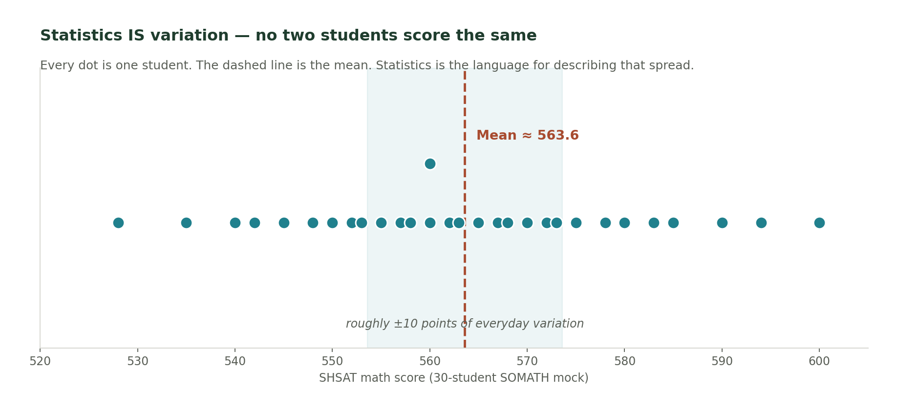
Ask a barista to pull twenty 30 mL espresso shots in a row. Weigh each one. You will get twenty different numbers — 29.6 mL, 30.2 mL, 29.4 mL, 30.1 mL, and so on — all clustered around 30 mL but none of them exactly equal to it. That spread is called variation, and it is the fundamental fact that motivates the entire discipline of statistics.
The one-sentence definition
Statistics is the science of collecting, describing, and drawing conclusions from data that varies. If every measurement were identical there would be no statistics course — one number would answer every question. The whole subject exists because repeated measurements are not identical.
Every unit of the AP Statistics course is a different lens on variation. Unit 1 (this unit) describes the variation in a single variable. Unit 2 describes how two variables vary together. Units 4 and 5 build a probability model for variation. Units 6, 7, 8, and 9 use that model to decide when observed variation is a real signal and when it’s just noise. If you keep “variation” as your north star, every unit will connect back to Class 1.
Population vs. sample, parameter vs. statistic
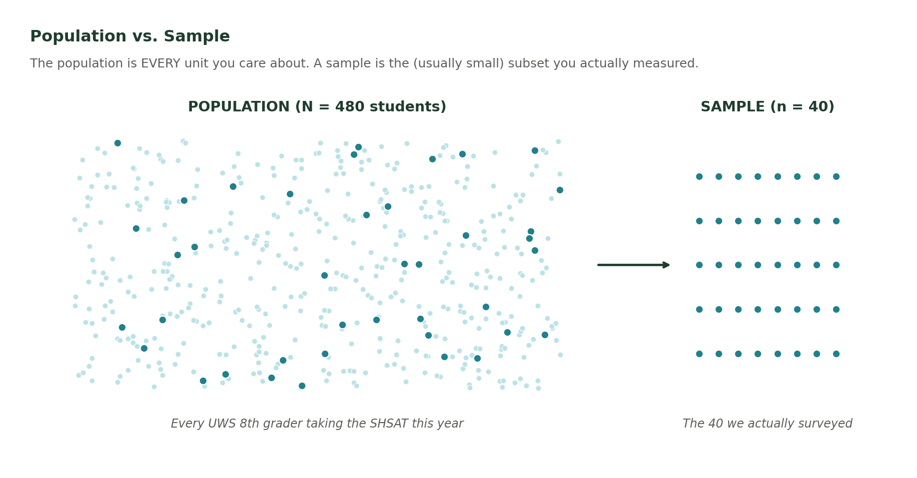
Almost every question in statistics has the same structure: there is a group I care about, and I want to know a number about that group, but I cannot measure the whole group so I measure a subset instead. The four words that name the pieces of that sentence appear in every AP Statistics free-response question you will ever solve.
The four-word vocabulary
- Population — the entire group you want to describe. Example: all 12-year-old girls in New York City.
- Sample — the subset of the population you actually measured. Example: 200 randomly chosen 12-year-old girls.
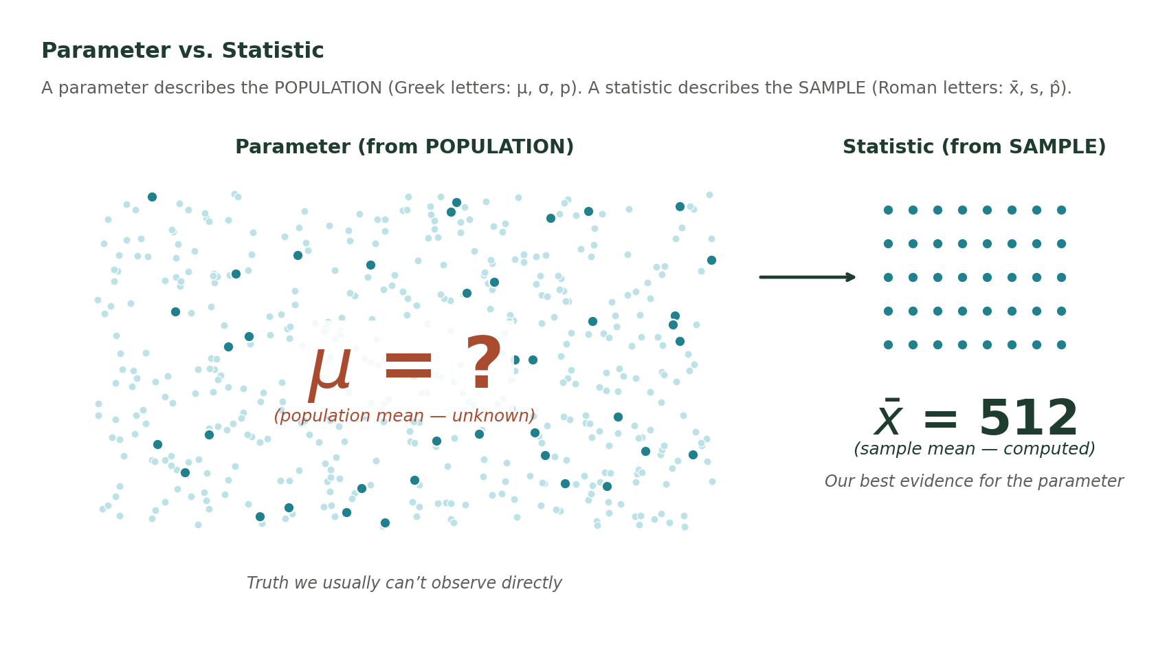
- Parameter — a true number describing the population. Usually unknown, denoted with Greek letters (μ for mean, σ for standard deviation, p for proportion).
- Statistic — a number computed from the sample. Usually known (you just measured it), denoted with Roman letters or hats (x̄ for sample mean, s for sample standard deviation, p̂ for sample proportion).
Every statistic estimates a parameter. The whole rest of the course — especially Units 6 through 9 — is a set of tools for saying how close the statistic is to the parameter.
Classifying variables: categorical vs. quantitative
Before you draw a single graph or compute a single number, you have to classify every column of your dataset. The classification determines which displays are legal (bar charts vs. histograms) and which summaries are legal (mode vs. mean).
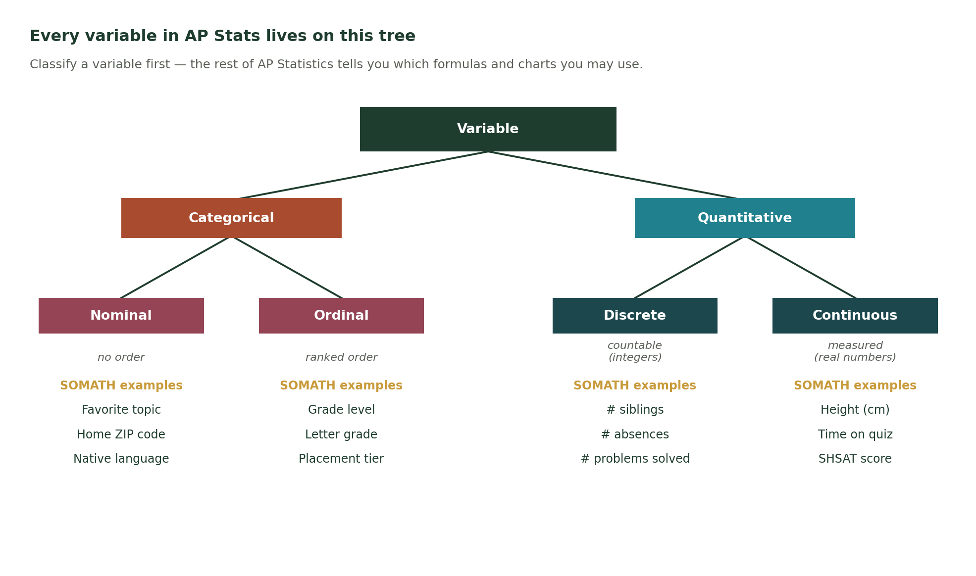
Categorical variables
A categorical variable takes values that are labels of groups, not amounts of anything. Examples: blood type (A / B / AB / O), preferred workout (cardio / weights / classes), whether a student takes AP Statistics (yes / no).
Categorical variables split into two sub-families:
- Nominal — the labels have no natural order. Blood type. ZIP code. Subway line.
- Ordinal — the labels have a natural order but not a numeric distance. T-shirt size (S < M < L < XL). Fitzpatrick skin scale (I through VI). Likert-scale survey ratings (1–5 satisfaction).
Quantitative variables
A quantitative variable takes numeric values on which arithmetic (adding, averaging, subtracting) has real-world meaning. Examples: height in cm, weekly income in dollars, number of siblings, time to run a mile.
Quantitative variables also split into two sub-families:
- Discrete — comes from counting in whole units. Number of siblings. Number of pepperoni slices. Goals scored.
- Continuous — comes from measuring on a scale where fractional values are possible. Height in cm. Time in seconds. Mass in grams. Temperature in °F.
Discrete vs. continuous quantitative variables
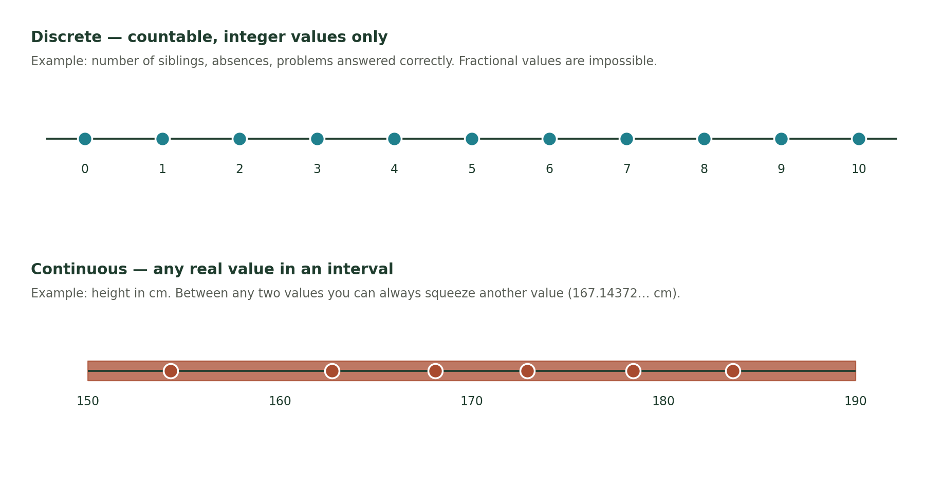
Once you know a variable is quantitative, the next question is which sub-family. The short version: counting is discrete, measuring is continuous.
The counting-vs-measuring test
Discrete quantitative variables are those you count in whole units. The set of possible values is a fixed grid (0, 1, 2, 3, ... or possibly negative integers) with no fractional values between grid points. Number of siblings, number of eggs in a carton, number of AP courses taken.
Continuous quantitative variables are those you measure on a scale where fractional values are always possible. Between any two heights (say 170.4 cm and 170.5 cm) there is another possible height (170.44 cm). With a better instrument you can always add more decimal places. Height, weight, time, mass, temperature, distance.
Class 1 recap — the vocabulary in one table
| Term | Meaning | Example |
|---|---|---|
| Population | The entire group you want to describe | All 12-year-old girls in NYC |
| Sample | The subset you actually measured | 200 randomly chosen 12-year-old girls in NYC |
| Parameter | A true number describing the population (usually unknown; Greek letters) | μ = true mean height of the population |
| Statistic | A number computed from the sample (Roman letters or hats) | x̄ = 152.4 cm sample mean |
| Categorical, nominal | Labels of groups, no order | Blood type, ZIP code, subway line |
| Categorical, ordinal | Labels with an order but no numeric distance | T-shirt size, Likert 1–5 rating |
| Quantitative, discrete | Counted in whole units | Number of siblings, goals scored |
| Quantitative, continuous | Measured on a scale allowing fractions | Height in cm, mile time in seconds |
Questions 1–8: Classify variables as categorical or quantitative
Eight short warm-ups on the single most important skill of Class 1: labeling every column in a dataset before you do anything else.
Question 1 · Categorical vs. Quantitative
A biology teacher records each student’s blood type (A, B, AB, or O). Is this variable categorical or quantitative?
Answer: Categorical
Key idea. A variable is quantitative only if arithmetic (adding, averaging) on its values makes sense. Blood type labels a group; you cannot compute a “mean blood type.”
Values: A, B, AB, O Can you add A + B? No. Can you compute an average? No. → Categorical (specifically, nominal — no natural order).Why this works. The blood-type labels are names of groups, not amounts of anything. Whenever the values are words (or codes standing in for words), start by suspecting categorical.
Question 2 · Categorical vs. Quantitative
A pediatrician records each child’s height in centimeters at the 5-year checkup. Is this variable categorical or quantitative?
Answer: Quantitative (continuous)
Key idea. A measurement in real units where arithmetic makes sense is quantitative. Height comes from a measuring device on a continuous scale.
Values: 108.4 cm, 112.1 cm, 105.7 cm, ... Mean height? Yes — adds and divides. Between any two heights there is another height → continuous. → Quantitative, continuous.Why this works. Anything you measure (length, weight, time, temperature) is quantitative continuous. Anything you count in whole units is quantitative discrete (Q3 next).
Question 3 · Categorical vs. Quantitative
A pizzeria records the number of pepperoni slices on each pie that leaves the oven. Is this categorical or quantitative?
Answer: Quantitative (discrete)
Key idea. You count pepperoni slices with whole numbers — you cannot have 12.7 slices. Counts are quantitative discrete.
Values: 12, 15, 14, 13, 16, 12, ... Mean = (12+15+14+13+16+12)/6 = 82/6 ≈ 13.67 slices per pie. The mean is not an integer, but the raw values are — that’s the discrete signature. → Quantitative, discrete.Why this works. The variable takes only integer values, but the summary statistics (mean, median) can be any real number. Discrete quantitative variables come from counting.
Question 4 · Categorical vs. Quantitative
A survey asks respondents: “On a scale of 1 to 5, how satisfied are you with your job?” The recorded value is the satisfaction rating. Categorical or quantitative?
Answer: Categorical (ordinal)
Key idea. Rating-scale answers look numeric but the numbers only label ordered categories. The gap between 1 and 2 is not guaranteed to equal the gap between 4 and 5. On the AP exam, treat these as categorical ordinal.
Values: 1, 2, 3, 4, 5 Is the “distance” between 1 and 2 the same as between 4 and 5? Not really — it depends on how each respondent felt. The values encode order, but not amount. → Categorical, ordinal.Why this works. Categorical variables split into nominal (blood type, no order) and ordinal (rating, T-shirt size — order but no true numeric distance). Ordinal variables are the classic AP trap.
Question 5 · Categorical vs. Quantitative
A middle school records each student’s ZIP code for the emergency contact form. Is ZIP code categorical or quantitative?
Answer: Categorical
Key idea. Even though ZIP codes look like numbers, arithmetic on them is meaningless — the average of 10024 and 10025 is not a real ZIP code you can mail to.
Values: 10024, 10025, 10023, ... Mean ZIP = (10024 + 10025 + 10023)/3 ≈ 10024. That number labels a neighborhood, not a “typical amount.” ZIP codes label geographic groups. → Categorical.Why this works. Ask: does arithmetic have real-world meaning? If no, it is categorical, even when the values are digits. Same idea for phone numbers, student ID numbers, and jersey numbers.
Question 6 · Categorical vs. Quantitative
A weather station records the daily high temperature in Fahrenheit at Central Park for each day of September. Categorical or quantitative?
Answer: Quantitative (continuous)
Key idea. Temperature is measured on a continuous scale; arithmetic (mean daily high, differences) is meaningful and standard.
Values: 78.4°F, 81.2°F, 76.9°F, ... Mean high for September = sum ÷ 30. Between 78.4 and 78.5 there are infinitely many possible values → continuous. → Quantitative, continuous.Why this works. Any physical measurement with a fractional scale is continuous quantitative. Temperature, height, weight, time, and distance all fall in this family.
Question 7 · Categorical vs. Quantitative
A subway operator records the train line letter (1, 2, 3, A, C, E, ...) for each trip. Categorical or quantitative?
Answer: Categorical
Key idea. The 1 train and the 2 train are labels for different subway lines. The “average” of the 1 line and the 3 line is not the 2 line in any meaningful sense.
Values: 1, 2, 3, A, C, E, ... Mixing digits and letters is a strong hint you are labeling groups, not measuring amounts. Mean line? No. → Categorical, nominal.Why this works. The digit-vs-letter mix is a give-away, but even the “pure number” version (Q5’s ZIP code) is still categorical. Focus on whether arithmetic makes sense, not on whether the raw value looks like a number.
Question 8 · Categorical vs. Quantitative
A researcher records each participant’s reaction time in milliseconds on a computer task. Categorical or quantitative?
Answer: Quantitative (continuous)
Key idea. Reaction time is a measurement on a continuous scale — you can always measure to more decimal places with a better clock.
Values: 312.4 ms, 287.1 ms, 405.6 ms, ... Mean, median, standard deviation all make sense. Any two reaction times have infinitely many possible values in between. → Quantitative, continuous.Why this works. Time-to-do-something is the canonical continuous quantitative variable in psychology and biology. The recording device’s precision is the only limit on the decimal places.
Questions 9–12: Discrete vs. continuous
Zoom in on quantitative variables and sort them into the two families: counts (discrete) and measurements (continuous).
Question 9 · Discrete vs. Continuous
For each of the following quantitative variables, mark it as discrete (D) or continuous (C): (a) number of siblings, (b) length of a car in meters, (c) exact time (in seconds) to run a mile, (d) number of goals scored in a soccer game.
Answer: (a) D, (b) C, (c) C, (d) D
Key idea. Discrete variables come from counting in whole units. Continuous variables come from measuring on a scale where fractional values are possible.
(a) Siblings: 0, 1, 2, 3, ... whole counts → Discrete. (b) Car length in meters: 4.32 m, 4.34 m, ... measured on a ruler → Continuous. (c) Mile time in seconds: 312.7 s, 312.71 s, ... measured on a stopwatch → Continuous. (d) Goals scored: 0, 1, 2, 3, ... whole counts → Discrete.Why this works. The one-word test: “Am I counting or am I measuring?” Counting → discrete. Measuring → continuous.
Question 10 · Discrete vs. Continuous
A survey asks each student for their shoe size (US women’s sizes: 6, 6.5, 7, 7.5, 8, ...). Discrete or continuous?
Answer: Discrete
Key idea. US shoe size is not a physical measurement in inches — it is a rounded label that only takes values on a fixed grid (every half-size). Between 7 and 7.5 there is no legal shoe size 7.2.
Legal values: 6, 6.5, 7, 7.5, 8, ... Between 7 and 7.5 there is no allowed value in this scheme. That gap-free requirement is the definition of continuous — and it fails. → Discrete.Why this works. Shoe size encodes a continuous measurement (foot length) but the recorded variable itself is discrete because it’s locked to a step grid. On the AP exam, always classify the recorded variable, not the underlying phenomenon.
Question 11 · Discrete vs. Continuous
A physics lab records the mass of a chemical sample to the nearest 0.01 gram. Discrete or continuous?
Answer: Continuous
Key idea. Mass is a continuous quantity in the real world, and rounding at the point of recording does not change the classification. The variable is still measured on a continuous scale.
Underlying quantity: mass (continuous). Recording precision: 0.01 g (a display limitation, not a hard grid of allowed values). With a better balance you would record 3.427 g, 3.4271 g, ... → Continuous.Why this works. Rounding is a property of the instrument, not of the variable itself. Contrast this with shoe size (Q10), where the grid is baked into the definition. Mass, length, and time are always continuous.
Question 12 · Discrete vs. Continuous
An ice-cream shop records the number of scoops sold each day. Discrete or continuous?
Answer: Discrete
Key idea. Counts of physical items are always discrete quantitative variables.
Values: 412, 508, 377, ... Can the count take fractional values? No — you cannot sell 412.7 scoops. Mean per day could be 432.15, but that’s a summary statistic, not a raw value. → Discrete.Why this works. The mean of a discrete variable can be non-integer, and that’s fine. The classification is based on what values the raw variable can take, not what the mean looks like.
Questions 13–15: Population vs. sample, parameter vs. statistic
The four-part vocabulary that carries you through the entire AP Statistics course — know it cold.
Question 13 · Population vs. Sample · Parameter vs. Statistic
A researcher wants to know the true average height of all 12-year-old girls in New York City. She measures 200 randomly chosen 12-year-old girls and computes their mean height to be 152.4 cm. Identify (a) the population, (b) the sample, (c) the parameter of interest, and (d) the statistic she computed.
Answer: (a) All 12-year-old girls in NYC. (b) The 200 measured girls. (c) The true mean height of the population (usually written μ). (d) The sample mean 152.4 cm (usually written x̄).
Key idea. The population is the full group you want to know about. The sample is what you actually measured. The parameter is the true (usually unknown) number describing the population; the statistic is the number you computed from the sample.
Question of interest: mean height of ALL 12-year-old NYC girls. (a) Population = all 12-year-old girls in NYC. (b) Sample = the 200 girls whose height was measured. (c) Parameter = μ = true mean height of the population (unknown). (d) Statistic = x̄ = 152.4 cm (computed from the sample). Statistic estimates parameter.Why this works. This four-part label is the vocabulary that carries you through the entire AP course. Every inference procedure in later units answers the question: how close is my statistic to the parameter?
Question 14 · Population vs. Sample · Parameter vs. Statistic
The US Census Bureau announces that 18.6% of Americans over 65 live alone, based on the complete 2020 census. Is 18.6% a parameter or a statistic?
Answer: Parameter
Key idea. The census measures the entire population, not a sample — so the resulting number describes the population directly and is a parameter.
The 2020 census attempts to reach every American, not a subset. When the count covers the entire population, the resulting summary is a parameter (denoted with Greek letters like μ, σ, p). → 18.6% is a parameter (specifically, the population proportion p).Why this works. The parameter/statistic label depends on who was measured, not on the size of the number. If it came from the whole population, it’s a parameter. If it came from a sample, it’s a statistic. In practice, true censuses are rare, so most numbers you meet are statistics.
Question 15 · Population vs. Sample · Parameter vs. Statistic
A Gallup poll of 1,022 randomly selected U.S. adults finds that 54% approve of the current mayor. Identify (a) the population, (b) the sample, (c) the parameter of interest, and (d) the statistic reported.
Answer: (a) All U.S. adults (or all U.S. adult voters, depending on the survey’s stated scope). (b) The 1,022 adults who were surveyed. (c) The true proportion p of all U.S. adults who approve of the mayor. (d) The sample proportion p̂ = 0.54.
Key idea. Same four-part decomposition as Q13, but for a proportion instead of a mean. The parameter is p; the statistic is p̂ (“p-hat”).
(a) Population = all U.S. adults (the group Gallup wants to describe). (b) Sample = the 1,022 randomly selected respondents. (c) Parameter = p = true proportion of U.S. adults who approve. (d) Statistic = p̂ = 0.54 = sample proportion. The headline “54%” is the sample statistic, not the true value.Why this works. In the news, sample statistics are almost always reported without their margins of error. Unit 6 comes back to this exact scenario to build a confidence interval that says how close p̂ is likely to be to p.
Questions 16–18: Variation, and why statistics exists
Three short conceptual questions on the deep “why” of the course: repeated measurements vary, and statistics is the language for that variation.
Question 16 · Variation & Why Statistics
A coffee shop’s espresso machine is supposed to pull a 30 mL shot. The barista pulls 20 shots in a row and gets: 29.6, 30.2, 29.4, 30.1, 30.5, 29.8, 29.9, 30.3, 29.7, 30.0, 30.4, 29.5, 30.1, 30.2, 29.8, 30.0, 29.6, 30.3, 29.9, 30.1 mL. Explain, in one sentence, why this is the reason statistics exists.
Answer: No two shots are exactly 30 mL — the values vary around the target — and statistics is the discipline that describes and reasons about that variation.
Key idea. If every measurement were identical, we would not need statistics. Statistics is the toolkit for describing, summarizing, and reasoning about the variation we see in repeated measurements.
Target: 30 mL. Observed values: 29.6, 30.2, 29.4, ... range from 29.4 to 30.5. Even though the machine is calibrated, no two shots match. That spread — the fact that repeated measurements are not identical — is what statistics studies.Why this works. The AP Statistics course opens with this idea because every unit that follows (distributions, sampling, inference) is a different lens on variation. If nothing varied, one measurement would answer every question.
Question 17 · Variation & Why Statistics
Two Manhattan pediatricians each measure the height of the same 6-year-old girl three times, five minutes apart. Doctor A gets 118.4, 118.7, 118.5 cm. Doctor B gets 118.2, 119.1, 118.6 cm. Which doctor’s measurements show more variability, and what does that tell you?
Answer: Doctor B’s measurements show more variability. That suggests Doctor B’s measuring technique (or ruler) is less consistent than Doctor A’s.
Key idea. For a fixed true height, the spread of repeated measurements reflects measurement variability. Less spread → more consistent (more precise) measurement.
Doctor A: 118.4, 118.7, 118.5 → range = 118.7 − 118.4 = 0.3 cm. Doctor B: 118.2, 119.1, 118.6 → range = 119.1 − 118.2 = 0.9 cm. Doctor B’s range is 3× larger. → Doctor B’s technique is less consistent.Why this works. This is the first appearance of a theme repeated all year: a summary is not complete without a spread. You never report just the center — you always report the variability with it.
Question 18 · Variation & Why Statistics
A student says: “My chemistry test scores this semester are 88, 92, 85, 90, 91, 87, 89, 93, 86, 91. The average is 89.2, so my typical score is 89.2 out of 100.” What is the student missing by reporting only the average?
Answer: The student is missing information about the variability (spread) of the scores. Two students with the same 89.2 average could have very different consistency — one might range from 85 to 93 (like this student), another from 60 to 100.
Key idea. The mean tells you the center of the data, but it does not tell you how spread out the data is. A full summary of a distribution requires both center and spread (and later, shape and outliers).
Data: 88, 92, 85, 90, 91, 87, 89, 93, 86, 91. Mean = 892 / 10 = 89.2. Range = 93 − 85 = 8. One student: 85 to 93 (range = 8) → consistent. Another student with the same 89.2 mean could score 60, 100, 70, 100, ... → very inconsistent. Same mean, very different stories. → Report center AND spread.Why this works. In Class 4 SOMATH students learn the SOCS framework (Shape, Outliers, Center, Spread) — the mandatory four-part description the AP exam requires. This question is the “why” for that habit.
Questions 19–20: Mixed applied practice
Two multi-part questions that combine everything in Class 1 and preview the survey-and-inference reasoning that shows up all year.
Question 19 · Mixed Applied
A dermatology clinic collects the following information for each patient: (a) age in years, (b) skin tone (Fitzpatrick scale I through VI), (c) whether they use sunscreen daily (yes / no), (d) number of moles on the left forearm, (e) SPF value of the sunscreen they use most often. Classify each variable as either categorical (nominal or ordinal) or quantitative (discrete or continuous).
Answer: (a) Quantitative discrete (age in whole years) — also acceptable: quantitative continuous if age is recorded to fractions of a year. (b) Categorical ordinal (I < II < III < IV < V < VI). (c) Categorical nominal (yes / no). (d) Quantitative discrete (count). (e) Quantitative discrete (SPF values are labeled 15, 30, 50, 70, 100 — a step grid).
Key idea. Real datasets mix all four variable types. Practice classifying every column before you touch a graph or a statistic — the classification determines which display and summary are legal.
(a) Age in years: whole-number count of years → Quantitative, discrete (or continuous if fractional). (b) Fitzpatrick scale: labels I–VI have order but not equal spacing → Categorical, ordinal. (c) Yes / No: two categories, no order → Categorical, nominal. (d) Number of moles: whole-number count → Quantitative, discrete. (e) SPF label: 15, 30, 50, 70, 100 (fixed grid) → Quantitative, discrete (some AP graders accept categorical ordinal — either is defensible).Why this works. Once you can label all the columns, you can pick displays: bar charts for (b) and (c), histograms for (a) and (d), and either display works for (e). Classification is the first step in every AP FRQ that gives you a dataset.
Question 20 · Mixed Applied
A gym is opening a new location on the Upper West Side and wants to describe its potential customer base. It has budget to survey 500 people who live within 10 blocks. Identify (a) the population, (b) the sample, (c) one categorical variable it might collect, (d) one quantitative variable it might collect, and (e) the difference between a parameter and a statistic in this context.
Answer: (a) Population = all people who live within 10 blocks of the new gym. (b) Sample = the 500 people the gym surveys. (c) Any variable like: preferred workout type (cardio / weights / classes / mixed), yes/no already a gym member, membership tier interest. (d) Any variable like: age in years, weekly hours currently spent exercising, monthly amount currently spent on fitness. (e) A parameter describes the population (unknown, e.g., the true mean age); a statistic describes the sample (computed from the 500 responses).
Key idea. Full walk-through of Class 1 vocabulary applied to a business decision. Every survey a real business runs is exactly this problem: use a sample to estimate a parameter of a population you cannot measure entirely.
(a) Population = all people within 10 blocks — the group the gym cares about but cannot survey in full. (b) Sample = the 500 people surveyed — the subset actually measured. (c) Categorical example: preferred workout type → values are labels (cardio, weights, classes). (d) Quantitative example: age in years → whole-number counts. (e) Parameter = true mean age of ALL 500-block residents (unknown). Statistic = mean age of the 500 surveyed respondents (computed). Business uses the statistic as its best guess for the parameter.Why this works. The reason SOMATH teaches AP Statistics as a life skill: this exact reasoning is what marketing teams, product managers, doctors, and journalists do every day. Learn the vocabulary in Class 1 and the rest of the course is a series of increasingly powerful tools built on it.
How SOMATH prepares NYC students for AP Statistics
SOMATH (School of Math) is a math-focused school on the Upper West Side of Manhattan, cofounded by Marcelo Ambrozio (Northwestern-trained lead math teacher) and Vivianne Wright (Harvard-trained). Our AP Statistics course is a full two-semester arc built for a 5 on the AP exam and for the analytical thinking students will use in every quantitative college class that follows.
Our AP Statistics track:
- Small-group in-person classes (6–8 students max) at 226 W 79th Street on the Upper West Side. Same room, same teacher, same students, week after week.
- Structured curriculum following the revised five-unit AP Statistics framework through SOMATH’s 24-class rolling syllabus, with current-format practice and written feedback.
- Calculator and Desmos fluency. Every student learns the TI-84 and Desmos statistics workflows: 1-Var Stats, LinReg, normalcdf, invNorm, tcdf, invT, and every inference procedure the exam expects.
- FRQ drilling with written feedback. Free-response questions from every released exam, graded on the actual AP rubric, with returned annotated rubrics.
- Free 30-minute in-person diagnostic evaluation before enrollment. A $99 one-time enrollment fee applies for new students who continue into a course.
Ready to build a 5 on AP Statistics?
Start with a free 30-minute in-person diagnostic at our Upper West Side classroom. Includes a written diagnostic report within 48 hours — yours to keep whether you enroll or not. A one-time $99 enrollment fee applies if you join a course.
Book Free Evaluation → or call (646) 668-6151
Want your child in an AP Statistics class at SOMATH?
Small-group AP Statistics preparation on the Upper West Side. Follow the revised five-unit framework, practice written interpretation, and begin with a free 30-minute evaluation.
AP Statistics Class 1 FAQ
What does AP Statistics Class 1 cover?
Class 1 introduces the whole discipline of statistics as the study of variation, defines the difference between a population and a sample, distinguishes a parameter (population) from a statistic (sample), and teaches how to classify any variable as categorical (nominal or ordinal) or quantitative (discrete or continuous).
How do I tell if a variable is categorical or quantitative?
Ask whether arithmetic on the values has real-world meaning. If you can compute a meaningful mean (like average height in cm), the variable is quantitative. If the values only label groups (like blood type or ZIP code), the variable is categorical, even when the labels look like numbers.
What is the difference between discrete and continuous quantitative variables?
Discrete variables come from counting in whole units (number of siblings, number of pepperoni slices). Continuous variables come from measuring on a scale where fractional values are possible (height in cm, time in seconds, mass in grams).
What is the difference between a parameter and a statistic?
A parameter is a number that describes an entire population (often unknown and denoted with Greek letters like μ or p). A statistic is a number computed from a sample (denoted x̄ for a sample mean or p̂ for a sample proportion). The whole point of statistical inference is to use statistics to estimate parameters.
Why does AP Statistics start with the idea of variation?
Because if repeated measurements were always identical there would be no need for statistics — one number would answer every question. Statistics exists to describe, summarize, and reason about the variation that shows up in real data, and every later unit (distributions, sampling, inference) is a different tool for handling variation.
How is SOMATH’s AP Statistics course structured?
SOMATH teaches AP Statistics in 2-hour classes on the Upper West Side of Manhattan. Unit 1 (Exploring One-Variable Data) is split into 8 classes: Class 1 (this page) covers variation and variable types, followed by displaying categorical data, displaying quantitative data, describing distributions with SOCS, summary statistics for center, summary statistics for spread and boxplots, the normal distribution and z-scores, and a review + assessment class.
Related posts
- Next class in the arc: AP Statistics Class 2 — Displaying Categorical Data
- Later in the arc: AP Statistics Class 11 — Random Variables & Expected Value — where the course transitions from data description into probability, with 60 original SOMATH practice questions.
- SOMATH SAT Math prep: Digital SAT Tutoring NYC 2026 — Structure, Dates & Scores
- Companion SAT walkthrough: Digital SAT Practice Test 9 — Math Module 1 Walkthrough
- SOMATH AP Statistics course page: See the AP Statistics course →
Continue with AP Statistics
Use this lesson alongside the AP Statistics course. For current exam preparation and related practice, start with these guides.